Interest-ing Calculations

John C. Nash 2023-4-1

** NOTE: The markdown rendering of this file is NOT correct. ***** See pdf link at https://web.ncf.ca/nashjc/BlogCopies/Interest-ingCalculations.pdf

All of us are affected by the interest charged or earned on money, but few people pay much attention to how the calculations are performed. Maybe they should, as there are many traps for the unwary. This article looks at a few of the issues and tries to clarify what can happen and how things should be done.

In passing, we note that various religions have had strictures concerning interest, generally under the term usury.

Simple interest calculations and rounding

The basic calculation of the interest I, the rent due on principal money P deposited or loaned at rate r is

I = P * r

Note that r is a fraction, not a percentage. In this article, we will use the symbol R for the nominal percentage interest per annum, as that is such a commonly used quantity that it deserves its own symbol. However, as we shall see later, this causes a number of difficulties.

A related quantity is the amount of money accumulated A:

A = (1+r)P

All this seems perfectly straightforward until you actually want your cash. Then you discover that

calculations (usually) need to be rounded to the nearest penny (in decimal currencies) before they can be recorded in a ledger;
if you want payment, there may be a smallest coin unit. In Canada this is the nickel (5 cent) piece. In the USA at 2023, it is still a penny (1 cent). See https://en.wikipedia.org/wiki/Cash_rounding for a list of different national practices.

Rounding is a subject that should be straightforward, but in reality is generally done poorly. Let us define a round to even algorithm.

Take the number to be rounded and split it after the last digit position to be kept. Let L be the digit to the left of the split and R be the number created by putting a decimal point in front of the digits to the right. If R is less than .5, leave L as is. If R is greater than .5, increase L by 1, carrying the increase left as needed. If R is exactly .5 (i.e. .500000 etc.), L is increased by 1 if it is odd, left as is if even.

Examples:
12.345 rounded to 2 decimal places or 4 figures is 12.34

12.345 rounded to 2 digits (0 decimals) is 12

12.345 rounded to 1 decimal (3 digits) is 12.3

12.350 rounded to 1 decimal (3 digits) is 12.4

A serious ERROR comes from cascade rounding, which I have seen students doing, and also arguing that their teachers taught them. This tries to do the following.

Suppose we want to round 1.234567 to 2 decimals (3 digits). The correct answer is to look at .4567 < 0.5 and round to 1.23.

Cascade rounding tries to do the following:

 1.234567 -> 1.23457 -> 1.2346 -> 1.235 -> 1.24  **WRONG**

While round-to-even is sometimes called “Banker’s rounding”, we would argue that it is the most common standard beyond the financial industry. However, readers should be aware that calculations may be executed with other rules, including truncation, which always returns L as the left hand digit regardless of the value of R.

Compound interest

Compound interest simply means we apply interest calculations repeatedly to a principal amount. For n periods, we end up with an amount

A = (1+r) * (1+r) * … * (1+r) * P = (1+r)ⁿ * P

The fun and games arise when we have a real-world bookkeeping situation and must report the amount at each time point where interest is accrued. What actually gets recorded will be the result A_n of a recursion

A_i + 1 = rounded[(1+r)*A_i]

where A₀ = P.

The rounded version of compound interest can deliver quite different amounts from the all-at-once or textbook formula.

ci <- function(P, er, n){ # all-at-once compound interest
  # P principal in cents, er effective rate (fraction), n periods
  A <- P * ((1 + er)^n )
}

cir <- function(P, er, n){
  # P principal in cents, er effective rate (fraction), n periods
  A <- P
  for (i in 1:n) {A <- round(A * (1 + er))}
  A  
}

er <- 3/100 # 3 % interest  
n  <- 20  # 20 periods (e.g., years)
pn <- 5
table <- matrix(NA, nrow=5, ncol=5)
for (j in 1:5) {
  P <- 10^j # Try different levels of principal
#  cat(P," cents at ", 100*er,"%  for ",n," periods gives ", ci(P, er, n),
#      " all-at-once or", cir(P, er, n)," rounded\n" )
  table[j,] <- c(P, 100*er,  ci(P, er, n), round( ci(P, er, n)), cir(P, er, n))
}
# put output in a table and have all-at-once rounded
colnames(table)<-c("P", "R", "textbook", "rd(textbook)", "rounded" )
print(table)

##          P R     textbook rd(textbook) rounded
## [1,] 1e+01 3     18.06111           18      10
## [2,] 1e+02 3    180.61112          181     179
## [3,] 1e+03 3   1806.11123         1806    1808
## [4,] 1e+04 3  18061.11235        18061   18061
## [5,] 1e+05 3 180611.12347       180611  180613

We see from the first row that it is possible to get no interest at all when we round. Yet simple interest over the 20 periods would give an amount

10 * (1 + (20*3/100) ) = 16 cents.

When interest rates are very low – and at the end of March 2023 TD Canada Trust is offering only 0.01% on savings accounts – the effects of rounding can be to eliminate all interest. As far as we can tell, this low rate is the per-annum rate (i.e., R) and not the per-day rate (i.e., 100 * r) in our description.

Minimum balance to earn daily interest over a 365 day year

Clearly, once rounding is in effect, we can have quite a lot of money in the bank and earn no interest, even on an account advertised as “Compound daily interest savings”. Moreover, the effect of rounding is such that a balance difference of 1 cent at the beginning of a year makes a great difference in the end-of-year balance. Let us explore this.

crdamt <- function(B, er, divn){ # Compound rounded interest for "year"
# B = balance in cents, er = fractional interest rate for "year", divn periods
  A <- B # amount in cents
  xer <- 0.01*er/divn
  for (i in 1:divn){
     A <- round(A*(1+xer))
  }
  A # amount in cents (smallest currency unit)
}

cmieb <- function(er, divn){ # Minimum interest earning balance
  xer <- 0.01*er/divn
  low <- 0 # lower bound
  up <- round(1/xer) # trial upper bound
  while (crdamt(up, er, divn) - up <= 0) {
     up <- 2*up+1 # ; cat("up=",up,"\n") # include if log wanted
  }
  count <- 1
  while ( up - low > 1 ) { #    cat("low and up", low, up,"\n")
     xx <- round(0.5*(low+up))
     vv <- crdamt(xx, er, divn) - xx
     if (vv == 0) { low <- xx }
     else {up <- xx} # choose up <- xx
     if (count >100) break # emergency exit
     count <- count+1
  }
  BC <- up # minimum balance that earns interest
}

divn <- 365
pcrv <- seq(0.01, 5, 0.01)
n <- length(pcrv)
balv<-rep(NA, n)
valint<-rep(NA, n)
for (i in 1:n){
  rate <- pcrv[i]
  balv[i] <- cmieb(rate, divn)
  valint[i] <- crdamt(balv[i], rate, divn)-balv[i]
}
plot(pcrv, balv)

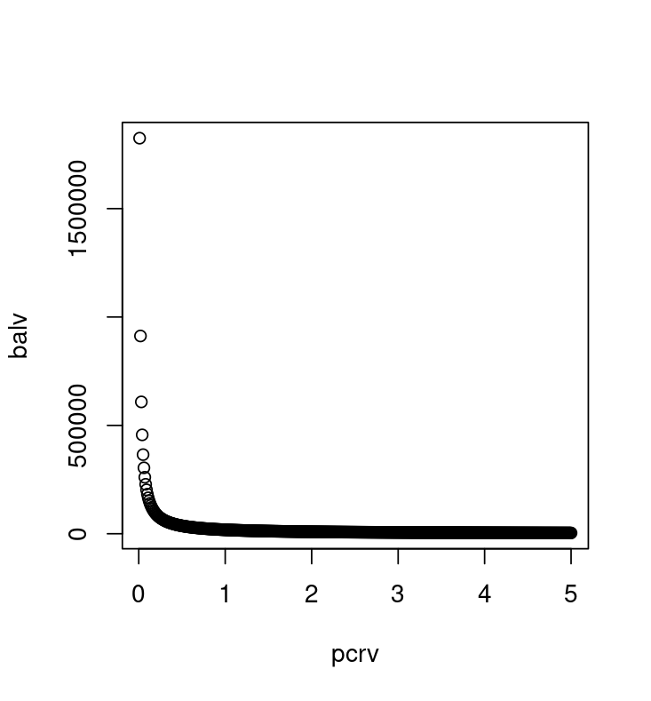
It turns out that the smallest non-zero interest paid will be a penny a day, or 365 cents, and this will be paid on the minimum interest earning balance. We note that this balance is 1825000 cents or $18,250 at the 0.01% interest rate quoted above. The minimum interest earning balance does not drop below $1000 until we are offered at least 0.19% per annum on a daily interest account. Why bother?!

Calendar annoyances

Calendars are a human construct to organize time. While the peculiarities of our solar system account for a lot of the difficulties with time division for interest calculations, humans have layered on more confusion.

Months can be from 28 to 31 days. This means a “half year” can be from 181 to 184 days. Of course, a 182.5 day half-year is equally awkward.

Generally monthly payments are made on the same numbered day of each month, even if the elapsed time between payments is unequal. The first of the month is a common choice. Note that the last day of the month gives different day-of-month numbers, but could be a choice.

A further complication is that we may want the first or last business day of the month. National, provincial/state or even municipal holidays then intervene to complicate matters.

Loan amortization

Loans are amortized or paid off in various ways. The most common and easiest to understand is the loan of principal P₀ at effective interest of 100 * r% per period for n periods. We can work out the per-period payment z.

First, in each period,

P_i + 1 = P_i * (1+r) − z

or more strictly

P_i + 1 = rounded(P_i*(1+r)−z)

For now ignore the rounding. We want to find z so that n payments give P_n = 0. But this is

P_n = 0 = P₀ * (1+r)ⁿ − z * ∑_{i = 1, n}((1+r)⁽ⁱ⁻¹⁾)

The right hand summation is a geometric progression. Its sum has a known formula, which we can easily derive.

Q = ∑_{i = 1, n}((1+r)ⁱ Q * ((1+r)−1) = r * Q = (1+r)ⁿ − 1) Q = [(1+r)ⁿ−1]/r

Giving

P₀ * (1+r)ⁿ * r/[(1+r)ⁿ−1] = z

z = P₀ * r/[1−(1+r)⁻ⁿ]

Thus the per-period payment for a loan of $10000 for 20 periods at 2% is

z <- 10000*0.02/(1 - 1.02^(-20))
z

## [1] 611.5672

Irregular amortization

Note that the usual convention is that payment is due at the END of each period, though there are many variations, and a lot of “pay-day” loans seem to front load the interest part of the payment at least, though they charge interest for the whole of the period.

Furthermore, rounding, business days or closings, delayed or early payments, extra or balloon payments, variable rate interest, or differing amortization and contract periods may alter the amount owing. Nevertheless, we can write the algorithm for the balance owing in full generality as

New_Principal = Payment_rule(Principal, rate(s), time_events)

If we slightly simplify so the rate for the period is r_i (in fractional form, not percentage, and applicable to the payment period), z_i is the current payment and f_i is the fraction of a regular payment period since the last reconciliation, then we get a new balance of

P_i + 1 = rounded(f_i*P_i*(1+r)−z_i)

Note that f_i is 1 for a regular payment interval, but could be larger or smaller depending on holidays, calendar effects, etc. Traditionally we did not see values for f_i other than 1. Similarly z_i was usually a fixed value approximated by the formula above for the per-period payment based on the number of amortization periods.

Contracts shorter than amortization period

The United States has commonly used mortgages that are contracted for the entire amortization period, typically 25 years or 300 months, with r = R/1200. British banks have been wary of intererst rate changes, and have treated mortgages as demand loans which are callable at any time. This would lead to a very disruptive process if people had to find ways to pay back the remaining mortgage balance at the whim of the bank. In practice, when rates change, the residue is computed i.e., a zero payment is presumed, then the next payment is made at a new rate for the (partial) period. Usually the bank communicates a different payment to the borrower.

Canada is, as usual, in between. Though variable rate mortgages are quite common (the situation just described for the UK, though likely using a modified narrative) fixed-rate mortgages in Canada generally have a shorter contract period, say 3 or 5 years, while the amortization period is 25 to 30 years. At the end of the contract, the borrower must repay the balance, typically by re-mortgaging a property i.e., recontracting the loan.

More Canadian quirks

A further oddity in Canada is that the Canada Interest Act (https://laws-lois.justice.gc.ca/eng/acts/i-15/page-1.html#h-270664) prescribes that mortgages shall be payable semi-annually or annually, not in advance. Of course, most householders prefer to pay monthly. This has led to a peculiar computation game that I believe is unique to Canada.

A way to think of this is that the lender (e.g., bank) accepts monthly payments and treats them as if they were deposits to a savings account at a fractional rate r that is such that the accumulated amount will be equal to the semi-annual payment.

Ignoring rounding, this is the same as using a monthly rate

r = (1+R/200)^1/6 − 1

We can check this with an example.

# semi-annual payment at 4% for 20 years on $100,000
z <- 100000*0.02/(1 - 1.02^(-40))
z # the payment value (unrounded)

## [1] 3655.575

r <- (1.02)^(1/6) - 1 # effective monthly rate
r # value

## [1] 0.00330589

# monthly payment at this rate on $100,000 for 20 years=240 months
q <- 100000*r/(1-(1+r)^(-240)) 
q # value

## [1] 604.2465

40 * z # total payout semi-annually 

## [1] 146223

240*q # total monthly pmts. Smaller because of earlier payment.

## [1] 145019.2

# check that value of 6 monthly payments is same as semi-annual
# payments calculated in reverse order of submission
# 0 months, 1, 2, 3, 4, 5 months interest earned
q+q*(1+r)+q*(1+r)^2+q*(1+r)^3+q*(1+r)^4+q*(1+r)^5

## [1] 3655.575

z # note the same value as computed before

## [1] 3655.575

We will not get into rounded computations here, but they are important when real mortgages in Canada are contracted. Unless the lender provides the borrower with a schedule of payments, the “rules” fall back to semi-annual or annual payments with a maximum rate prescribed at 5%.

Weekly mortgages

There have been occasional fashions for weekly mortgages. These present yet another issue, particularly in Canada. First, several reasonable mechanisms for the computation of the effective per period fractional rate r can be proposed. In the mid-1980s I did discover at least 2 ways used by different financial institutions. Second, there are calendar issues in reconciling the weekly payments with “semi-annual”.

A possible set of rules

As mentioned, financial institutions may put forth many different rules. Most are likely acceptable, but some are almost certainly unfair to borrowers in that the conditions and calculation algorithms are not clearly laid out. Here are some specifications I would recommend.

interest rates should be stated in per-annum values R with documented algorithms for computing the effective per-period fractional rate r.
the number of compounding periods in a year should be given clearly
the timing of payments should be specified, if necessary including the time zone, along with rules for dealing with holidays or business closing days, as well as exceptions.
for partial periods, simple interest on the fractional period should be used, that is, the interest due should be $ P * r * (f) $ where f is the fraction of the period.
interest is paid or due at the end of each payment period i.e., not in advance.

Written on April 1, 2023